Flights Analysis
The goal of this post is to visualize flights taken from Google location data using Python * We will create a .gif progressing through individual flights and a .png of all flights * This post utilizes code from Tyler Hartley’s visualizing location history blog post
Overview
- Setup
- download data
- install modules
- Data Wrangling
- data extraction
- data exploration
- data manipulation
- Flight Algorithm
- Visualize Flights
- create individual .png of each flight to combine into .gif
- create .png of all flights plotted at once
- Conclusion
Setup
- Use Google Takout to download your Google location history
- If you’ve previously enabled Google location reporting on your smartphone, your GPS data will be periodically uploaded to Google’s servers. Use Google Takeout to download your location history.
- The decisions of when and how to upload this data are entirely obfuscated to the end user, but as you’ll see below, Android appears to upload a GPS location every 60 seconds. That’s plenty of data to work with.
- After downloading your data, install the required modules
Google Takeout
Google Takeout is a Google service that allows users to export any personal Google data. We’ll use Takeout to download our raw location history as a one-time snapshot. Since Latitude was retired, no API exists to access location history in real-time.
Download location data: * Go to takeout. Uncheck all services except “Location History” * The data will be in a json format, which works great for us. Download it in your favorite compression type. * When Google has finished creating your archive, you’ll get an email notification and a link to download. * Download and unzip the file, and you should be looking at a LocationHistory.json file. Working with location data in Pandas. Pandas is an incredibly powerful tool that simplifies working with complex datatypes and performing statistical analysis in the style of R. Chris Albon has great primers on using Pandas here under the “Data Wrangling” section.
Install modules
- If you use Anaconda to manage your Python packages, I recommend creating a virtual environment with anaconda to install the dependencies. Copying the lines below the instruction into the terminal creates the environment, requirements.txt, etc.
- conda create -n test-env python=3.5 anaconda
- source activate test-env
- make a requirements.txt file for dependencies
- (echo descartes; echo IPython; echo shapely; echo fiona; echo Basemap) >> requirements.txt
- install requirements.txt
- conda install –yes –file requirements.txt
- Windows users:
- create a python2.7 environment to install relevant modules
- conda create -n py27 python=2.7 anaconda
- source activate py27
- Download and install Microsoft Visual C++ Compiler for Python 2.7
- install fiona, Shapely, GDAL, descartes, and basemap from https://www.lfd.uci.edu/~gohlke/pythonlibs/
After completing the setup, we’ll read in the LocationHistory.json file from Google Takeout and create a DataFrame.
Data Wrangling
Explore Data
accuracy                     int64
activity                    object
altitude                   float64
heading                    float64
latitude                   float64
longitude                  float64
timestamp                  float64
velocity                   float64
verticalAccuracy           float64
datetime            datetime64[ns]
dtype: object
| count |
745660.000000 |
101260.000000 |
44100.000000 |
745660.000000 |
745660.000000 |
7.456600e+05 |
58874.000000 |
4921.000000 |
| mean |
58.997173 |
67.057525 |
186.597551 |
37.748367 |
-102.506537 |
1.417774e+09 |
7.769678 |
23.099776 |
| std |
125.358984 |
242.209547 |
101.643968 |
9.004123 |
23.609836 |
3.356510e+07 |
11.790783 |
45.139324 |
| min |
1.000000 |
-715.000000 |
0.000000 |
13.689757 |
-123.260751 |
1.376790e+09 |
0.000000 |
2.000000 |
| 25% |
22.000000 |
-18.000000 |
98.000000 |
29.817569 |
-122.306596 |
1.391259e+09 |
0.000000 |
2.000000 |
| 50% |
31.000000 |
2.000000 |
181.000000 |
29.986634 |
-95.246060 |
1.413249e+09 |
1.000000 |
2.000000 |
| 75% |
50.000000 |
60.000000 |
270.000000 |
47.664284 |
-94.995603 |
1.428049e+09 |
13.000000 |
30.000000 |
| max |
999.000000 |
6738.000000 |
359.000000 |
50.105984 |
23.782015 |
1.519330e+09 |
208.000000 |
473.000000 |
- accuracy code “999” may represent missingness
- find earliest and latest observations in the data
earliest observed date: 08-17-2013
latest observed date: 02-22-2018
Data manipulation
Degrees and Radians
- We’re going to convert the degree-based geo data to radians to calculate distance traveled. I’m going to paraphrase an explanation (source below) about why the degree-to-radians conversion is necessary
- Degrees are arbitrary because they’re based on the sun and backwards because they are from the observer’s perspective.
- Radians are in terms of the mover allowing equations to “click into place”. Converting rotational to linear speed is easy, and ideas like sin(x)/x make sense.
Consult this post for more info about degrees and radians in distance calculation.
convert degrees to radians
calculate speed during trips (in km/hr)
Make a new dataframe containing the difference in location between each pair of points.
Any one of these pairs is a potential flight
Now flightdata contains a comparison of each adjacent GPS location.
All that’s left to do is filter out the true flight instances from the rest of them.
spherical distance function
- distance_on_unit_sphere: function to calculate straight-line distance traveled on a sphere
- see utils.py for function documentation
Flight algorithm
- filter flights
- remove flights using conservative selection criteria
This algorithm worked nearly 100% of the time for me with less than 5 false positives or negatives; however, the adjacency-criteria of the algorithm is fairly brittle. The core of it centers around the assumption that inter-flight GPS data will be directly adjacent to one another. That’s why the initial screening on line 1 of the previous cell had to be so liberal.
Now, the flights DataFrame contains only instances of true flights which facilitates plotting with Matplotlib’s Basemap. If we plot on a flat projection like tmerc, the drawgreatcircle function will produce a true path arc just like we see in the in-flight magazines.
Visualize Flights
Reset the flight index and change index values by adding a leading 0 for index items 0-9 (e.g., 1 becomes 01)
This new index is important for correctly ordering images as we create a gif
view the first observation in the flights dataframe
level_0                                  114
index                                     00
distance                             255.032
end_datetime      2013-09-08 11:00:26.190000
end_lat                              30.4372
end_lon                             -95.4975
speed                                117.789
start_datetime    2013-09-08 08:50:31.631000
start_lat                            32.4222
start_lon                           -96.8384
Name: 00, dtype: object
Create .gif and .png of all flights
- Create a folder called
flights2018 within the output directory to save all .pngs
- Loop through each flight and create a .png with the following characteristics
- the origin of the current flight is a green circle
- the destination of the current flight is red circle
- the current flight is gold
- previous flights are purple
- the origin and destination of previous flights are black circles
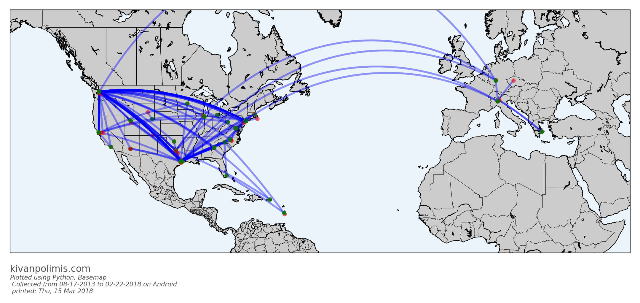
- The .png of all flights loops through the flights data frame and plots each flight simultaneously
- create a .gif by combing all the (ordered) .pngs in the
flights2018 directory with the glob
- use ImageMagick to create the .gif
- ImageMagick is a free and open-source software suite for displaying, converting, and editing raster image and vector image files. It can read and write over 200 image file formats.
- source: https://en.wikipedia.org/wiki/ImageMagick
- create .png of all flights
- Calculate all the miles you have traveled in the years observed with a single line of code:
172130.0 miles traveled from 08-17-2013 to 02-22-2018
Conclusion
You can leverage this notebook, scripts, and cited sources to reproduce these maps.
I’m working on creating functions to automate these visualizations
Potential future directions
- label airports
- add flight information (origin, destination, etc.) in the legend of each .png that is used to create the .gif
Download this notebook, or see a static view here
System and module version information:

Python version:
 sys.version_info(major=2, minor=7, micro=14, releaselevel='final', serial=0)

last updated: Thu, 15 Mar 2018 04:28
Source: Flights Analysis
Flights Analysis
The goal of this post is to visualize flights taken from Google location data using Python * We will create a .gif progressing through individual flights and a .png of all flights * This post utilizes code from Tyler Hartley’s visualizing location history blog post
Overview
- Setup
- download data
- install modules
- Data Wrangling
- data extraction
- data exploration
- data manipulation
- Flight Algorithm
- Visualize Flights
- create individual .png of each flight to combine into .gif
- create .png of all flights plotted at once
- Conclusion
Setup
- Use Google Takout to download your Google location history
- If you’ve previously enabled Google location reporting on your smartphone, your GPS data will be periodically uploaded to Google’s servers. Use Google Takeout to download your location history.
- The decisions of when and how to upload this data are entirely obfuscated to the end user, but as you’ll see below, Android appears to upload a GPS location every 60 seconds. That’s plenty of data to work with.
- After downloading your data, install the required modules
Google Takeout
Google Takeout is a Google service that allows users to export any personal Google data. We’ll use Takeout to download our raw location history as a one-time snapshot. Since Latitude was retired, no API exists to access location history in real-time.
Download location data: * Go to takeout. Uncheck all services except “Location History” * The data will be in a json format, which works great for us. Download it in your favorite compression type. * When Google has finished creating your archive, you’ll get an email notification and a link to download. * Download and unzip the file, and you should be looking at a LocationHistory.json file. Working with location data in Pandas. Pandas is an incredibly powerful tool that simplifies working with complex datatypes and performing statistical analysis in the style of R. Chris Albon has great primers on using Pandas here under the “Data Wrangling” section.
Install modules
- If you use Anaconda to manage your Python packages, I recommend creating a virtual environment with anaconda to install the dependencies. Copying the lines below the instruction into the terminal creates the environment, requirements.txt, etc.
- conda create -n test-env python=3.5 anaconda
- source activate test-env
- make a requirements.txt file for dependencies
- (echo descartes; echo IPython; echo shapely; echo fiona; echo Basemap) >> requirements.txt
- install requirements.txt
- conda install –yes –file requirements.txt
- Windows users:
- create a python2.7 environment to install relevant modules
- conda create -n py27 python=2.7 anaconda
- source activate py27
- Download and install Microsoft Visual C++ Compiler for Python 2.7
- install fiona, Shapely, GDAL, descartes, and basemap from https://www.lfd.uci.edu/~gohlke/pythonlibs/
After completing the setup, we’ll read in the LocationHistory.json file from Google Takeout and create a DataFrame.
Data Wrangling
Explore Data
accuracy                     int64
activity                    object
altitude                   float64
heading                    float64
latitude                   float64
longitude                  float64
timestamp                  float64
velocity                   float64
verticalAccuracy           float64
datetime            datetime64[ns]
dtype: object
| count |
745660.000000 |
101260.000000 |
44100.000000 |
745660.000000 |
745660.000000 |
7.456600e+05 |
58874.000000 |
4921.000000 |
| mean |
58.997173 |
67.057525 |
186.597551 |
37.748367 |
-102.506537 |
1.417774e+09 |
7.769678 |
23.099776 |
| std |
125.358984 |
242.209547 |
101.643968 |
9.004123 |
23.609836 |
3.356510e+07 |
11.790783 |
45.139324 |
| min |
1.000000 |
-715.000000 |
0.000000 |
13.689757 |
-123.260751 |
1.376790e+09 |
0.000000 |
2.000000 |
| 25% |
22.000000 |
-18.000000 |
98.000000 |
29.817569 |
-122.306596 |
1.391259e+09 |
0.000000 |
2.000000 |
| 50% |
31.000000 |
2.000000 |
181.000000 |
29.986634 |
-95.246060 |
1.413249e+09 |
1.000000 |
2.000000 |
| 75% |
50.000000 |
60.000000 |
270.000000 |
47.664284 |
-94.995603 |
1.428049e+09 |
13.000000 |
30.000000 |
| max |
999.000000 |
6738.000000 |
359.000000 |
50.105984 |
23.782015 |
1.519330e+09 |
208.000000 |
473.000000 |
- accuracy code “999” may represent missingness
- find earliest and latest observations in the data
earliest observed date: 08-17-2013
latest observed date: 02-22-2018
Data manipulation
Degrees and Radians
- We’re going to convert the degree-based geo data to radians to calculate distance traveled. I’m going to paraphrase an explanation (source below) about why the degree-to-radians conversion is necessary
- Degrees are arbitrary because they’re based on the sun and backwards because they are from the observer’s perspective.
- Radians are in terms of the mover allowing equations to “click into place”. Converting rotational to linear speed is easy, and ideas like sin(x)/x make sense.
Consult this post for more info about degrees and radians in distance calculation.
convert degrees to radians
calculate speed during trips (in km/hr)
Make a new dataframe containing the difference in location between each pair of points.
Any one of these pairs is a potential flight
Now flightdata contains a comparison of each adjacent GPS location.
All that’s left to do is filter out the true flight instances from the rest of them.
spherical distance function
- distance_on_unit_sphere: function to calculate straight-line distance traveled on a sphere
- see utils.py for function documentation
Flight algorithm
- filter flights
- remove flights using conservative selection criteria
This algorithm worked nearly 100% of the time for me with less than 5 false positives or negatives; however, the adjacency-criteria of the algorithm is fairly brittle. The core of it centers around the assumption that inter-flight GPS data will be directly adjacent to one another. That’s why the initial screening on line 1 of the previous cell had to be so liberal.
Now, the flights DataFrame contains only instances of true flights which facilitates plotting with Matplotlib’s Basemap. If we plot on a flat projection like tmerc, the drawgreatcircle function will produce a true path arc just like we see in the in-flight magazines.
Visualize Flights
Reset the flight index and change index values by adding a leading 0 for index items 0-9 (e.g., 1 becomes 01)
This new index is important for correctly ordering images as we create a gif
view the first observation in the flights dataframe
level_0                                  114
index                                     00
distance                             255.032
end_datetime      2013-09-08 11:00:26.190000
end_lat                              30.4372
end_lon                             -95.4975
speed                                117.789
start_datetime    2013-09-08 08:50:31.631000
start_lat                            32.4222
start_lon                           -96.8384
Name: 00, dtype: object
Create .gif and .png of all flights
- Create a folder called
flights2018 within the output directory to save all .pngs
- Loop through each flight and create a .png with the following characteristics
- the origin of the current flight is a green circle
- the destination of the current flight is red circle
- the current flight is gold
- previous flights are purple
- the origin and destination of previous flights are black circles
- The .png of all flights loops through the flights data frame and plots each flight simultaneously
- create a .gif by combing all the (ordered) .pngs in the
flights2018 directory with the glob
- use ImageMagick to create the .gif
- ImageMagick is a free and open-source software suite for displaying, converting, and editing raster image and vector image files. It can read and write over 200 image file formats.
- source: https://en.wikipedia.org/wiki/ImageMagick
- create .png of all flights
- Calculate all the miles you have traveled in the years observed with a single line of code:
172130.0 miles traveled from 08-17-2013 to 02-22-2018
Conclusion
You can leverage this notebook, scripts, and cited sources to reproduce these maps.
I’m working on creating functions to automate these visualizations
Potential future directions
- label airports
- add flight information (origin, destination, etc.) in the legend of each .png that is used to create the .gif
Download this notebook, or see a static view here
System and module version information:

Python version:
 sys.version_info(major=2, minor=7, micro=14, releaselevel='final', serial=0)

last updated: Thu, 15 Mar 2018 04:28